It is simple to calculate confidence intervals in R. There’s no function in base R that will just compute a confidence interval, but we can use the z.test and t.test functions to do what we need here (at least for means – we can’t use this for proportions).
If we know the population standard deviation, we can use the z.test() function (from the BSDA package) to construct the confidence interval. We supply the population standard deviation and the confidence level to the function as follows:
library("BSDA") test1 z.test(choc, sigma.x = 2, conf.level = 0.95) test1$conf.int## [1] 39.94773 40.02613 ## attr(,"conf.level") ## [1] 0.95If we do not know the population standard deviation, which is most often the case in practice, we typically use the t.test() function (included in base R). In this case we will only supply the confidence level, and the function will use the standard error to construct the interval.
test2 t.test(choc, conf.level = 0.95) test2$conf.int## [1] 39.94724 40.02661 ## attr(,"conf.level") ## [1] 0.95The interpretation of confidence intervals can be summarised as follows: if repeated samples were taken from the population and the 95% confidence interval computed for each sample, 95% of the intervals would contain the population mean in the long run. Let’s see if we can simulate what this statement implies through the example below.
Say we send a bunch of people to the chocolate factory to sample and measure the mean weight of the chocolate bars. They each take a sample of 20 bars, and construct a 95% confidence interval from their sample. For example, the following would be one possible realization of a confidence interval computed in this manner:
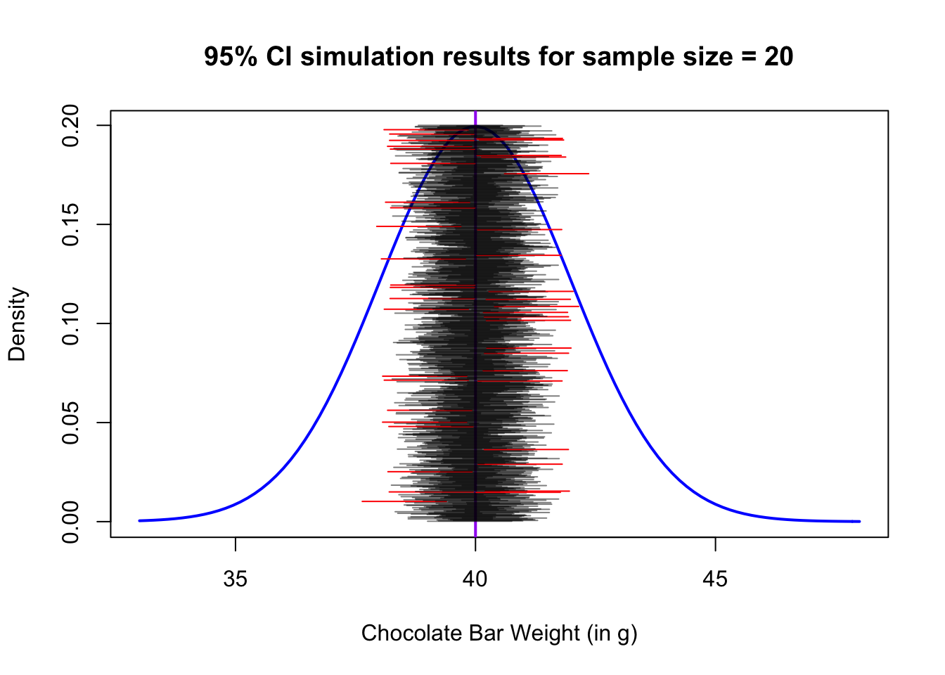
choc.batch rnorm(n = 20, mean = 40, sd = 2) test3 z.test(choc.batch, sigma.x = 2, conf.level = 0.95) test3$conf.int## [1] 38.73064 40.48369 ## attr(,"conf.level") ## [1] 0.95Let’s tally how many of their confidence intervals covered, or included, the true mean. The following code simulates the process of repeatedly sampling batches of 20 bars from the true distribution, and constructing confidence intervals from each sample. One thousand batches are sampled in the code below. (Don’t worry about the large block of code, we will not expect you to plot things like this, but it is an illustration of what R is capable of. There is also a function in the BSDA package called CIsim that does a similar thing).
attempts = 1000 curve(expr = dnorm(x, mean = 40, sd = 2), from = 33, to = 48, main = "95% CI simulation results for sample size = 20", xlab = "Chocolate Bar Weight (in g)", ylab = "Density", lwd=2, col="blue") abline(v = 40, col = "purple", lwd = 2) failed_to_contain 0 for (i in 1:attempts) rgb(0,0,0,0.5) choc.batch rnorm(n = 20, mean = 40, sd = 2) myCI z.test(choc.batch, sigma.x = 2, conf.level = 0.95)$conf.int if (min(myCI) > 40 | max(myCI) 40) failed_to_contain + 1 col rgb(1,0,0,1) > segments(min(myCI), 0.2 * i / attempts, max(myCI), 0.2 * i / attempts, lwd = 1, col = col) >
This illustrates how the confidence intervals are correct a prespecified percentage of the time, and that percentage is known as the confidence level.
In this case, for a 95% confidence interval, notice that approximately 5% of the confidence intervals we constructed actually DO miss the true mean (the ones in red).
failed_to_contain / attempts## [1] 0.044